Taking a closer look at the radar effect shown in SNDH v4.8 update demo

Table Of Contents
You can either download the demo and watch it in your (emulated) machine of choice, or you can look at the YouTube capture below.
Flying in enemy territory (Premise)
In early 2020, in that wretched hive of scum and villainy called IRC, Grazey and GGN were discussing plans about making an intro for the final SNDH update. Initially, the whole demo was going to be just the second part of the demo released. Grazey was on top of that (in all fairness, it was his project anyway), so some discussions happened on a few technical issues that aren’t too relevant for this article.
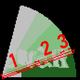
Late February, an idea came to Grazey’s mind. What if there was a small sequence at the beginning that resembled a radar and introduced all the groups involved into the production? The following video was used as an inspiration:
GGN was asked if this would be possible. “It would just be a few fading lines, sure” was the vague answer. After all, the duo have used a rather awkward line routine for Trans D-bug Express, so it should have been a breeze.
Some more work happened during Tathack where GGN and Grazey were together in the same place.
Falling off the radar (Development slows down)
After Tathack, the Covid-19 lockdowns happened. So a few things (including the intro) were put on hold. Long story short, Grazey and GGN kept working on it, but in different time periods, so development was slow.
But eventually both sat down at the same time period (around December 2022) and cranked through all the unfinished items and released the intro. For various reasons, the release happened on February 2023, but the work for the intro was finished one month earler.
Vicious circle (Circle go brrrrrr)
The reasonable/easy/realistic thing to do would have been to draw some fading lines over a black screen (with maybe the outline of an island or a terrain) and display some spots in various parts of the lines’ path and then maybe print some text (or display some logos). But, inspiration being the thing that it is, it was decided that the terrain itself would be the logos of the groups, fading in and out as the radar moved. So, quite suddenly, the difficulty bar was raised. Textured lines were in the discussion table.
Before even get to the coding part began, an interesting question arose: How to fill a circle fast? This matters because the radar effect had to to move fast enough. A full revolution of the lines shouldn’t take more than a few seconds, otherwise the effect will lose its dynamism (you are free to rewatch the final version of the intro, and notice how frantic the pacing of the sound effects are. That pace was desired, so it was locked as a design input)
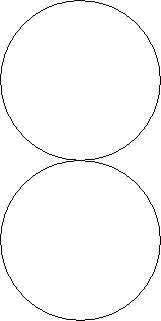
Assuming almost zero knowledge of the subject, why not revisit those geometry lessons from high school? The teachers would say that a full circle’s revolution is 360 degrees. So let’s try drawing 360 lines, one per each degree. This is the result:

It’s fast at least, but it’s really not great. The gaps really don’t give the impression of a filled circle. So, keeping the naiveness, we try a step value smaller than 1 degree:

A bit better, but still not perfect. Let’s use an even smaller step value:

Still not perfect, let’s try an even smaller value:

Perfect! Except, notice how slow it fills the circle compared to the first experiment. This is obviously a problem. But how to fix this?
One idea would be to draw multiple lines per frame, so that there will be no visible gaps (actually, that’s the approach that the line routine of Trans D-Bug Express went with). However, this would not be feasible here due to the amount of lines to be drawn - it would easily run in less than 50 frames per second, and neither of the two people wanted that. Another (even worse reason) is that there would be more than one line drawn on screen, so this would be magnitudes slower than the desired frame rate.
Another idea would be to draw filled circle arcs instead of lines. So that way would ensure no gaps occur and the speed would be adjustable; just change the length of the arc and it the effect would run faster or slower. This was never tried because again it was deemed that it would slow the effect down by a lot.
Yet another idea that was not tried was to use the so called Midpoint circle algorithm (also known as Bresenham cirlce algorithm). This one has the peculiarity of drawing 8 segments, with different directions, simultaneously. It is very suited to drawing a circle very fast, but not great for drawing parts of a circle, which is what was wanted. Also, it is quite probable that this algorithm is also prone to the Moire patterns shown above.
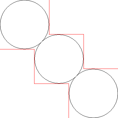
At this point GGN remembered of an old article he read more than two decades ago, written by a certain Mr Eugen Dedu. The article’s name is Bresenham-based supercover line algorithm [archived here for posterity](/static/circle/Bresenham modified algorithm - ALL the points.mhtml)
(Foreshadowing: Make a note of this picture, as it will come back to haunt some of the decisions down the line)
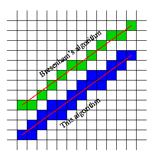
It was in intriguing article, as it looked as if it could be handy for getting rid of jaggies in lines. Sure, some accuracy might be sacrificed in certain angles (the line in blue above seems a bit more blocky than the ideal green one). But with fast moving lines it hopefully would not be very visible. What if this algorithm was applied with radial lines?

This looks near perfect, and doesn’t take that long to do a full revolution, success! Here is a side-by-side comparison between the supercover algorithm and two other (naive) step values:

Probably a bit slower than the one-degree-step circle, but still acceptable. (Eventually this method became even faster than the 1 degree step value)
Avoiding getting spotted (Prototyping the effect)
Still at the prototyping stage, and not wanting to go and program the effect in full assembly so it would look bad, the effect was prototyped in a high level language. (For the curious, it is GFA BASIC 32. Because old habits die hard)
Some logos drawn by ST Survivor were available, so those were crudly converted to greenscale and got shrunk a bit in order to fit the circle boundaries (which at that time had a radius of 80 pixels, so 160 pixels wide/high).
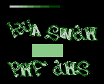
First of all, since it was very possibly going to be too hard to do all the fades in real time, the logos had to be faded up to full white and down to full black. So the above image was transformed into this:
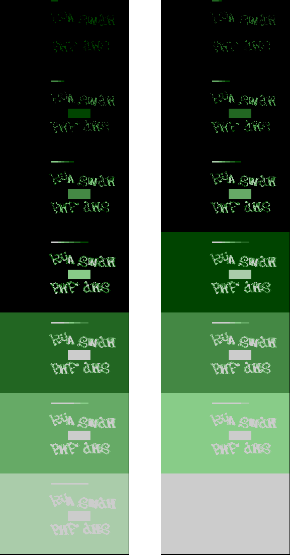
It is now “only” a matter of picking segmnents in the form of lines from each of the 14 images, plot it to the destination buffer and…

It doesn’t look that great? At that point panic started settling in. If the lines had to be spread apart, shouldn’t this mean that all lines between the whitest and blackest line had to be drawn?
It turns out that no, it doesn’t:
The trick is visible at the start of the animation above: If the lines are drawn more far apart, there will be a certain amount of frames that they will have the same intensity before they will need to be faded down. So, by simply drawing 14 lines (plus another one which is fully black) with some degrees apart between each other, the illusion of fading out is preserved.
Under the radar (The things we do to get pixels on screen)
After all this initial work, it was time to start considering how the actual code that runs on the ST is going to look.
Starting again with a naive approach, just to show a sense of complexity, here is a possible routine that draws a single pixel on an ST low resolution 4 bitplane screen: (the discussion about ST bitplanes will have to wait for another article, as this one is going to be long enough without this)
; Assuming that d0=x coordiant and d1=y coordinate.
; d7 is the colour (0 to 15)
; a0 is the address of the top-left pixel.

mask_tab:
        dc.w    $7fff,$bfff,$dfff,$feff,$f7ff,$fbff,$fdff,$feff
        dc.w    $ff7f,$ffbf,$ffdf,$ffef,$fff7,$fffb,$fffd,$fffe

plot_pixel:
        move.w  d0,d2
        and.w   #15,d2
        lsr.w   #1,d0
        and.w   #%1111111111111000,d0
        mulu    #160,d1
        add.w   d1,d0
        lea     (a0,d1.w),a0
        add.w   d7,d7
        move.w  mask_tab(pc,d7.w),d5
        move.w  d5,d6
        not.w   d6
        lsl.w   #3,d7
        jmp     plot_routines(pc,d7.w)

plot_routines:
        and.w   d5,(a0)+
        and.w   d5,(a0)+
        and.w   d5,(a0)+
        and.w   d5,(a0)+
        rts
        ds.w    3

        or.w    d6,(a0)+
        and.w   d5,(a0)+
        and.w   d5,(a0)+
        and.w   d5,(a0)+
        rts
        ds.w    3

        and.w   d5,(a0)+
        or.w    d6,(a0)+
        and.w   d5,(a0)+
        and.w   d5,(a0)+
        rts
        ds.w    3

        or.w    d6,(a0)+
        or.w    d6,(a0)+
        and.w   d5,(a0)+
        and.w   d5,(a0)+
        rts
        ds.w    3

        and.w   d5,(a0)+
        and.w   d5,(a0)+
        or.w    d6,(a0)+
        and.w   d5,(a0)+
        rts
        ds.w    3

        or.w    d6,(a0)+
        and.w   d5,(a0)+
        or.w    d6,(a0)+
        and.w   d5,(a0)+
        rts
        ds.w    3

        and.w   d5,(a0)+
        or.w    d6,(a0)+
        or.w    d6,(a0)+
        and.w   d5,(a0)+
        rts
        ds.w    3

        or.w    d6,(a0)+
        or.w    d6,(a0)+
        or.w    d6,(a0)+
        and.w   d5,(a0)+
        rts
        ds.w    3

        and.w   d5,(a0)+
        and.w   d5,(a0)+
        and.w   d5,(a0)+
        or.w    d6,(a0)+
        rts
        ds.w    3

        or.w    d6,(a0)+
        and.w   d5,(a0)+
        and.w   d5,(a0)+
        or.w    d6,(a0)+
        rts
        ds.w    3

        and.w   d5,(a0)+
        or.w    d6,(a0)+
        and.w   d5,(a0)+
        or.w    d6,(a0)+
        rts
        ds.w    3

        or.w    d6,(a0)+
        or.w    d6,(a0)+
        and.w   d5,(a0)+
        or.w    d6,(a0)+
        rts
        ds.w    3

        and.w   d5,(a0)+
        and.w   d5,(a0)+
        or.w    d6,(a0)+
        or.w    d6,(a0)+
        rts
        ds.w    3

        or.w    d6,(a0)+
        and.w   d5,(a0)+
        or.w    d6,(a0)+
        or.w    d6,(a0)+
        rts
        ds.w    3

        and.w   d5,(a0)+
        or.w    d6,(a0)+
        or.w    d6,(a0)+
        or.w    d6,(a0)+
        rts
        ds.w    3

        or.w    d6,(a0)+
        or.w    d6,(a0)+
        or.w    d6,(a0)+
        or.w    d6,(a0)+
        rts
        ds.w    3
(Again, please note that the above code is for illustrative purposes only. I did not attempt to run or debug this code. However, if you feel adventurous and try it out, and spot bugs, please use the feedback form at the bottom to mention them and they shall be corrected.)
This is not a completely naive implementation. It does have some jump tables and also the masks and plot values are read from a table. But this is far from performant code, and trying to plot a few hundreds of pixels using code would result in really slow runtime.
There are a few main problems with the above piece of code:
- The address inside the screen buffer is calculated every time, which takes a lot of time. That
muludoes a multiplication which is quite slow. Also the shift operationslsrandlslare not exactly the fastest. - There are 16 different routines, of which only one is called depending on the colour value that
d7contains. Because in general the previous value of the specific pixel on screen is not known, the code cannot assume anything and has to operate on all four bitplanes. So for each pixel 4x the work is required. - There are also some other things that are not visible here. Since this will be called many times from somewhere just to draw a line (which, by coincidence, is composed of many pixels laid out in a specific order), even more control logic is required.
There are some easy ways to mitigate the first pain point, and this will certainly bring some savings to the table.
- A line is composed of dots that are strictly one next to each other (as the illustration from the supercover algorithm above shows), the screen address of the first pixel of each line can be calculated. Also, since all lines start from the same point (the centre of the circle), this will be a common and fixed value for all lines
- Since some adds and shifts are used for the jump table and reading mask values off the first table, the value in
d7could be precalculated so those arithmetic operations are not required - Each subsequent pixel from the centre one will be one pixel apart. So the screen address and pixel inside the bitplane can be calculated as a difference from the previous. This is much less expensive than all the multiplications and shifts
- A common optimisation in drawing lines is the assumption that a pixel will move along one axis, or the other, or both, but never in the opposite direction. That is, if a line has a slope which is to the top right from its origin point, each subsequent pixel from the origin will strictly move right, up, or up-right. It will never move left or down. This can be used to simplify the line control code a lot
Running circles around (can we do better?)
The above optimisations are all fine and well, they certainly help to speed up the overall implementation. But the elephant in the room still has not been addressed. Namely:
Those awful AND/OR quartets
Without even trying to measure performance, those awful sets of instructions are already burning 4x more bandwidth that anyone would want. How could this be mitigated?
At this point, it is a good idea to zoom in a bit at the plot code, but from a different angle. The following table illustrates the above ANDs and ORs that are required to plot the pixels on screen:
| Colour \ Bitplane | 1 | 2 | 3 | 4 |
|---|---|---|---|---|
| 0 | X | X | X | X |
| 1 | O | X | X | X |
| 2 | X | O | X | X |
| 3 | O | O | X | X |
| 4 | X | X | O | X |
| 5 | O | X | O | X |
| 6 | X | O | O | X |
| 7 | O | O | O | X |
| 8 | X | X | X | O |
| 9 | O | X | X | O |
| 10 | X | O | X | O |
| 11 | O | O | X | O |
| 12 | X | X | O | O |
| 13 | O | X | O | O |
| 14 | X | O | O | O |
| 15 | O | O | O | O |
(X means that the bitplane is off, O means that the bitplane is on)
This illustrates the problem with our approach. Assuming that our brightest pixel is pixel 15 and our darkest pixel 0, there are problems with the transitions from the first to last states. Namely (assuming that pixel value 15 is drawn already):
- To get from the state of pixel 15 to the state of pixel 14 bitplane 0 has to be set to off
- To get from the state of pixel 14 to the state of pixel 15 bitplane 0 has to be set to on, and bitplane 2 has to be set to off
- etc etc
The thing to state again at this point is that the only way the pixels are going to change is from value 15 to 0. From the above table It is really easy to notice that the state changes don’t necessarily change all bitplanes every step. So there is already a big win from that observation; rewrite the plot routines with the minimal amount of code required to change from one state to the other.
Could this idea be optimised further?
Yes.
Up till now the transitions were done in a naive way to match the numbers 15 to 0 in binary format. So, as stated above, the amount of state changes is not fixed. But as it turns out, more clever people (while solving different problems) came up with a way to reduce the number state changes into a fixed number, namely one:
While nothing revolutionary for this day and age, Gray codes produce sequences of binary numbers that successive values have only one state change different. So, the above table can be rearranged like this:
| Colour \ Bitplane | 1 | 2 | 3 | 4 |
|---|---|---|---|---|
| 0 | X | X | X | X |
| 8 | X | X | X | O |
| 12 | X | X | O | O |
| 4 | X | X | O | X |
| 6 | X | O | O | X |
| 14 | X | O | O | O |
| 10 | X | O | X | O |
| 2 | X | O | X | X |
| 3 | O | O | X | X |
| 11 | O | O | X | O |
| 15 | O | O | O | O |
| 7 | O | O | O | X |
| 5 | O | X | O | X |
| 13 | O | X | O | O |
| 9 | O | X | X | O |
| 1 | O | X | X | X |
With the colours ordered that way it is very easy to notice that (assuming a totally zeroed out buffer) drawing colour 16 (1) means that we simply have to set bitplane 1 to on. Likewise, going from the 16th colour (1) to the 15th (9) we only require to set bitplane 4. Similarly, to go from colour 15 (9) to 14 (13) we just need to set bitplane 3. And so on and so forth. Finally, notice that the last colour (0) has all bitplanes cleared, so we can then cycle back to colour 15 (1) without any overhead.
This is indeed more tangible! It is certainly unorthodox, and will require that the palette is swizzled compared to normal plotting of pixels. But luckily the hardware doesn’t care, it will happily convert that jumbled mess into a sequence of fading colours, and now the code is 7 times faster than before (because before there were 4 AND and 4 OR instructions, while now there is only one AND or OR). Victory!
On the radar (Further complications)
Time to write some code then? Not quite…
It is time to visualise what was briefly mentioned a few paragraphs above about drawing lines. The following illustrations show a typical line with a more horizontal slope and a more vertical one.
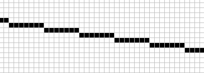
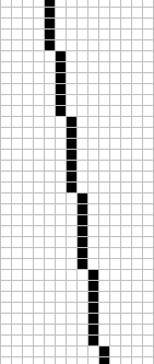
One way to draw the horizontal line is to start at the leftmost point, and then keep moving horizontally for every subsequent pixel, and in certain occasions move upwards one pixel. Likewise for vertical: Start at the topmost pixel, then keep going down one pixel and occasionally one pixel to the right. This is fairly easy to implement and not too bad on computation costs.
Therefore, in order to draw a line we simply have to store its length, initial position, and slope. Then the line routine has enough information to go draw.
It’s now time to revisit the supercover algorithm line image from earlier.
This totally violates the above assumptions about how to draw this line; to go to the next pixel we could move right, up-right or up-left.
Not good.
For lack of a better solution, the directions can be encoded in a bitfield. Therefore, for each pixel of each line the relative movement can be stored and then the line drawing routine can decode that and know how to move.
| Bit | 7 | 6 | 5 | 4 | 3 | 2 | 1 | 0 |
|---|---|---|---|---|---|---|---|---|
| Direction | n/a | n/a | n/a | n/a | Up | Down | Left | Right |
Practically, for each line a series of bytes that describe the movement will be stored. This solution covers all 8 possible directions. Of course there is waste here as half the byte goes unused, but this can be fixed as long as the performance is fine (for example, the 4 unused bits can store movement for another pixel).
Move in the right circles (The last piece of the puzzle)
One last thing to consider before sitting down and writing the actual assembly code.
So far we discussed how to plot pixels efficiently. And this would have been enough if it weren’t for the little fact that we wish to draw textured lines, where each pixel value can be different from the previous. What would be a good way to do that?
At this point all the experts would unanimously exclaim “Just use a chunky buffer, bro!”. And we shall just do that. Every pixel value shall be encoded using the quirky Gray code table above, and with the needed palette adjustments (which also won’t reflect an order than a normal person would expect) it should be fine.
There is a subconscious nag at this point about memory consumption. After all, each pixel is now a single byte instead of 4 bits (so, a 50% space increase right off of the bat) repeated 14 times because of the fading (see the big bitmap above in Avoidng getting spotted). Which means 28 times more than the original pixel value. This is a concern, but there are still so many unknowns in the implementation that this will be addressed in due time (i.e. “Design”).
Squaring the circle (Time to get busy)
After all that legwork, it is finally time to write some code that will run on the actual hardware. The tool exports the images in chunky data, and the line segments in the format described above. Code is written to match the exported data and visualise it on screen. What could go wrong?
Well…
…it does run. But, that flickering background is well known in demo circles as a bad sign. It means that the code takes more than one Vertical Blank to execute. Which means that the 50 FPS constraint that was was defined at the start, the one that caused all this research to happen, is now being violated.
The nine circles of Hell (Disaster recovery mode)
Cold sweat.
(for a few seconds)
Deep breath. Regroup. Think.
Go back and review the code. The plotting part itself seems fairly optimal. Apart from the fact that the chunky table still contains pixel values that have to be converted into jump offsets. This can be a big performance hit due to the amount of pixels plotted. This works because the plot code is small enough that the jumps fit inside one byte. This is an easy gain. So the tool is modified to output jump offsets.
What else could be optimised?
How about the movement table? That part of the code is not that great, since there are a lot of decisions to be taken during runtime:
- Each direction checked means that a
btstinstruction has to be used. If the code is laid out in a smart way, a few tests can be skipped, but still this means branches - The code has to keep track of the bitplanes. If the current pixel is in a bitplane boundary (either leftmost or rightmost bit) and the next pixel is outside that boundary, then the address needs to also be adjusted and some offsets reset. This is especially bad since most of the tests are false for the generic case.
- (An implementation detail is that pixels are plotted using
bset Dn,y(Am)/bclr Dn,y(Am)instead ofor.w Dn,y(Am)/and.w Dn,y(Am)for reasons that won’t be explained here. Point being, this also could have an extra computational cost added to the above)
Is there some way that all the above decisions would go away? How about a jump table?
Going back to the line movement table (described in On the radar), for each pixel a single byte is output, and it was noted that it’s wasteful. How can the above be converted to a jump table?
- The tool can be fed with the exact coordinates that will be shown on the actual screen
- While the tool calculates the next pixel’s position, it can keep track of the direction and convert that into an offset to a routine that is specialised for that movement. This gets rid of all
btstinstructions - Since the tool also knows the coordinates, it also can calculate when bitplane boundary jumps happen and can point to an extra set of routines that adjust screen address and reset the counters, as stated above
The resulting table points to a set of routines that do the exact amount of work required for moving to the next pixel, and the only cost is one branch instead of multiple (and unknown)
So all the above ideas are fed into the tool, the tool crunches the numbers and writes out a new set of tables, the assembly code is modified to incorporate all the changes and…
… not that bad?
Coming full circle (What’s left?)
Around this point the effect became tangible. There were a few other optimisations that happened before or after the above optimisation pass, like the first and last lines being solid black or white, so two specialised routines were written to remove the plot table complexity. This also contributed to some of the speed gains.
Luckily (?) a discussion between GGN and Grazey revealed that the actual circle radius was to be 60 pixels (120 pixels diameter) instead of 80. This brought back a lot of CPU time, so no further optimisations were needed. However, if needed the effect could be optimised further.
Probably the most profitable optimisation left (but not explored) is to change slightly the way the line routine works. Observing the effect in action, it is quickly observed that each drawn line has a dominant colour, plus variations to form the logo. Thus it can be split into three parts:
- From the centre point to the first point that the logo starts for that line
- From the start of the logo to the end of the logo (again, going radially from the centre to the end point)
- From the end of the logo to the end point of the circle
The first and last parts have the same pixel value, thus they can use a specialised routine that plots a specific pixel value, without plot jumps. This should give a fair amount of performance back.
Another possible optimisation has to do with memory management. Currently, the chunky buffers are laid out in memory in this fashion:
This is fine, but since we use a square texture and just use the pixels of a circle inscribed in a square. This is not a fully fleshed out idea, but we should be able to do a different layout of the data:
This should release some unused parts of RAM.
Eventually it was decided that the team shouldn’t try to make the demo run in 512k (there are only so many rabbit holes one can fall into), so this thread was abandoned.
Circling the drain (Things not covered)
As is the norm with these kinds of write ups, there are many things that were omitted in an attempt to contain the size of this text. A few of them shall be briefly mentioned below.
- From the state the effect is left to the final version there was a lot of work that happened. As mentioned before, keeping multiple 160x160x14 byte textures in RAM so they can then be swapped to show the logos as in the final version was considered very wasteful. So instead each logo was stored (along with its faded versions) stand alone as smaller squares. Then a single 160x160x14 byte chunky canvas was reserved. The demo sequencer then had to copy and clear the logos when they were outside the visible area. This of course is synced with the beeping sound effect, which gave birth to a sequencer that counted the number of vertical blank ticks and queued drawing and clearing of logos (note that more than one logo could have been drawing simultaneously, to keep up with the pace. So in a sense there was some multitasking happening).
- Funnily enough, the screen does not swap screens. A balance was struck that reduces screen tearing to a minimum, so everything is racing the beam per frame.
- Integration with a different codebase is always a pain point. Since both Grazey and GGN worked independently of each other, the time came where the two codebases had to be merged. Anticipating that, GGN had make his code be as easy to integrate as possible, and with the exception of a few hiccups and misunderstandings in Grazey’s code, the process was fairly smooth.
- Because Grazey wrote most of the code as a quick proof of concept to explain the design of the screen, the code was fairly unoptimised. GGN, during integration, spotted that and had to re-code some ciritcal routines. The name plotters were optimised using Gray code tricks, so overall CPU usage dropped to around 1/5th to 1/10th of what it originally took.
- The accompanying track actually uses a SID voice or the beep. This has been measuered to take peak 11% CPU time. Again, this didn’t become a problem as there was more than that left after all the oprimisations were in place.
- As a stretch goal, Grazey decided to add some screen shakes (like in the original reference video) on the screen just to spice things up. This proved a very good choice, as the whole effect became more dynamic. A little trivia about this: The shakes happen on a timer (which of course means more CPU time drainage) and there are 4 different code paths for STF, STE, TT and Falcon, which all produce different effects. Especially the STF codepath, due to changing screen frequency at completely random points, makes the effect visible only in tolerant CRT monitors - TFT monitors and capture equipment have a really hard time keeping up.
The radar (In conclusion)
It could be argued that, due to the amounts of optimisation this effect underwent, it has become an animation. This is purely subjective of course, and every person has their own standards of what is realtime and what isn’t. One opinion is that the effect:
- Is programmable, i.e. any chunk of graphics can be displayed using it, at any position, at any time
- Would take magnitudes more RAM if it was a pure (packed) animation
- The pixels are drawn and erased per frame, so it’s not something pre-fabed
Taking the above points into consideration, it is logical to deduce that the effect is not an animation. However, there are is a definition of animation along the lines of “a super efficient packer designed for a single effect”, which whould classify most modern demos as animations. Again, it is up to each person to judge for themselves.